Ordinary Least Squares (OLS) Regression
Author: Bindeshwar Singh Kushwaha
Institute: PostNetwork Academy
Dataset of a Company
| X (Budget) | Y (Sales) |
|---|---|
| 1 | 2 |
| 2 | 2.8 |
| 3 | 3.6 |
| 4 | 4.5 |
| 5 | 5.1 |
Description:
- The dataset represents the relationship between advertising budget (\(X\)) and sales revenue (\(Y\)).
- The company wants to analyze how the budget affects sales using regression analysis.
- The goal is to fit a regression model to predict sales based on the budget.
Ordinary Least Squares (OLS) Regression
Definition: OLS is a statistical method used to estimate the relationship between independent and dependent variables by minimizing the sum of squared residuals.
Objective: Find the best-fit line:
\[ Y = \beta_0 + \beta_1 X + \epsilon \]
where:
- \( Y \) = Dependent variable (response)
- \( X \) = Independent variable (predictor)
- \( \beta_0 \) = Intercept (value of \( Y \) when \( X = 0 \))
- \( \beta_1 \) = Slope (change in \( Y \) per unit change in \( X \))
- \( \epsilon \) = Error term (residuals)
Minimizing the Error: The goal is to minimize the sum of squared errors (SSE):
\[ SSE = \sum (Y_i – \hat{Y}_i)^2 \]
Solution: The OLS estimates for \( \beta_1 \) and \( \beta_0 \) are:
\[ \beta_1 = \frac{\sum (X_i – \bar{X})(Y_i – \bar{Y})}{\sum (X_i – \bar{X})^2}, \quad \beta_0 = \bar{Y} – \beta_1 \bar{X} \]
Calculation of \( \beta_1 \) and \( \beta_0 \)
Step 1: Compute \( \beta_1 \)
\[ \beta_1 = \frac{7.90}{10.00} = 0.79 \]
Step 2: Compute \( \beta_0 \)
\[ \beta_0 = \bar{Y} – \beta_1 \bar{X} \]
\[ \bar{X} = \frac{1+2+3+4+5}{5} = 3, \quad \bar{Y} = \frac{2+2.8+3.6+4.5+5.1}{5} = 3.42 \]
\[ \beta_0 = 3.42 – (0.79 \times 3) = 3.42 – 2.37 = 1.05 \]
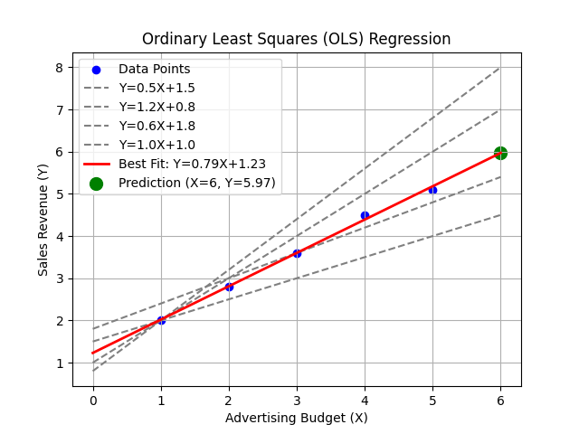
Final Regression Equation:
\[ Y = 1.05 + 0.79X \]
Prediction on Unseen Data using \( Y = 0.79X + 1.05 \)
Step 1: Given the Regression Equation
\[ Y = 0.79X + 1.05 \]
Step 2: Choose an Unseen Value of \( X \)
Suppose we want to predict sales (\( Y \)) for an advertising budget of \( X = 6 \).
Step 3: Substitute \( X = 6 \) into the Equation
\[ Y = 0.79(6) + 1.05 \]
Step 4: Compute the Predicted Value
\[ Y = 4.74 + 1.05 = 5.79 \]
Step 5: Interpretation
- If the company spends \( X = 6 \) on advertising, it is expected to generate \( Y = 5.79 \) in sales.
- This prediction is based on past trends observed in the dataset.
- The closer the test data is to the training data, the more reliable the prediction.
Video
import numpy as np
import pandas as pd
import statsmodels.api as sm
import matplotlib.pyplot as plt

# Define dataset
X = np.array([1, 2, 3, 4, 5])  # Advertising Budget
Y = np.array([2, 2.8, 3.6, 4.5, 5.1])  # Sales Revenue

# Convert X to a DataFrame and add a constant for the intercept
X = sm.add_constant(X)  # Adds a column of ones to estimate the intercept

# Fit the OLS model
model = sm.OLS(Y, X).fit()

# Print the regression summary
print(model.summary())

# Plot the data and regression line
plt.scatter(X[:, 1], Y, label='Data Points', color='blue')
plt.plot(X[:, 1], model.predict(X), label='Best Fit Line', color='red')
plt.xlabel("Advertising Budget")
plt.ylabel("Sales Revenue")
plt.legend()
plt.title("OLS Regression: Budget vs Sales")
plt.show()

# Predict sales for an advertising budget of 6
X_new = sm.add_constant(np.array([6]))
Y_pred = model.predict(X_new)
print(f"Predicted Sales for Budget 6: {Y_pred[0]:.2f}")
Reach PostNetwork Academy
- Website: www.postnetwork.co
- YouTube: www.youtube.com/@postnetworkacademy
- Facebook: www.facebook.com/postnetworkacademy
- LinkedIn: www.linkedin.com/company/postnetworkacademy