 Here’s a line-by-line explanation of the LaTeX code:
1. `\documentclass[10pt,aspectratio=169]{beamer}`
– This line specifies the document type as a Beamer presentation.
– `10pt`: Sets the font size to 10 points.
– `aspectratio=169`: Specifies the aspect ratio of the slides (16:9, which is a widescreen format).
2. `\usepackage[applemac]{inputenc}`
– This imports the `inputenc` package and specifies the character encoding as “Apple MacRoman”, which is typically used for documents with special characters typed on a Mac system.
3. `\usepackage[T1]{fontenc}`
– This ensures that the document uses “Type 1 fonts” for better output, especially for accented characters and special symbols.
4. `\usepackage{lmodern}`
– This package loads the “Latin Modern” font, which is a modern version of the Computer Modern font that LaTeX uses by default. It improves font appearance, especially in PDFs.
5. `\usetheme{Madrid}`
– This line specifies the “theme” for the Beamer presentation, which in this case is “Madrid”. This theme controls the style of the slides, including colors, font size, and layout.
6. `\usepackage{ragged2e}`
– This package allows text alignment, particularly enabling “justified or ragged-right text”.
7. `\usepackage{graphicx}`
– This package is used to “include graphics” in the document, such as images and figures.
8. `\begin{document}`
– This marks the “start” of the document content.
9. `\author{Bindeshwar Singh Kushwaha}`
– This defines the “author” of the presentation.
10. `\title{Calculating Variance of Continuous Frequency Distribution}`
– This defines the “title” of the presentation.
11. `\subtitle{Data Science and A.I. Lecture Series}`
– This adds a “subtitle”to the presentation.
12. `\institute{PostNetwork Academy}`
– This specifies the “institution” of the author, which in this case is “PostNetwork Academy”.
13. `\date{}`
– This sets the “date” of the presentation. The empty curly braces mean that no date will be displayed.
14. `\begin{frame}[plain]`
– This starts a new “frame” (or slide) with the `[plain]` option, meaning the frame will not include any default navigation symbols or decorations.
15. `\maketitle`
– This command “generates the title slide”, displaying the title, subtitle, author, and institution.
16. `\end{frame}`
– This ends the current “frame” (slide).
17. `\begin{frame}{Reach PostNetwork Academy}`
– This begins a new “frame” (slide) titled “Reach PostNetwork Academy”.
18. Inside the frame:
– Each `\begin{block}{}` creates a **block** with the specified title, and the contact details for PostNetwork Academy are displayed as text inside these blocks.
“`latex
\begin{block}{Website}
PostNetwork Academy | www.postnetwork.co\\
\end{block}
“`
– The `\\` creates a line break after the website link.
19. The frame includes blocks for:
– Website
– YouTube Channel
– Facebook Page
– LinkedIn
20. `\begin{frame}`
– This starts another frame (slide), which contains a **table** that will show how to calculate the variance of a continuous frequency distribution.
21. Inside the frame:
– `\centering`: Centers the content on the slide.
– `\begin{block}{}`: Creates a block around the table.
– `\begin{tabular}{|c|c|c|c|c|c|c|}`: This line defines a table with 7 columns, each separated by a vertical bar `|`. Each `c` means the column is centered.
22. `\uncover<1->{}`:
– `\uncover` makes specific parts of the slide appear on specific slide transitions. The number “ inside the brackets controls when the content appears as the slide is shown.
– In this case, it delays revealing parts of the table row by row as the presentation progresses.
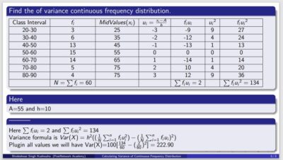
23. Table Content:
– The table shows various columns such as:
– Class Interval: The intervals for the data.
– $f_i$: Frequency for each class interval.
– $x_i$: Midpoint of each class interval.
– $u_i = \frac{x_i – A}{h}$: The formula for calculating a transformed value of each midpoint using the average \( A \) and step size \( h \).
– $f_i u_i$: The product of frequency and the transformed value.
– $u_i^2$: Square of the transformed value.
– $f_i u_i^2$: The product of frequency and the square of the transformed value.
24. Data Rows:
– Each row of the table shows the corresponding data for different class intervals, with `\uncover` delaying parts of each row to be revealed in sequence.
25. `N=\sum f_i = 60`
– This calculates the **total frequency** by summing up the frequencies $f_i$.
26. Variance Calculation:
– A block explains how the variance is calculated.
– Given values:
– \( A = 55 \) (the assumed mean).
– \( h = 10 \) (the class width).
– The **variance formula** is:
\[
Var(X) = h^2 \left( \frac{1}{N} \sum_{i=1}^{n} f_i u_i^2 – \left( \frac{1}{N} \sum_{i=1}^{n} f_i u_i \right)^2 \right)
\]
– Substitute values
– The sum of $f_i u_i$ is 2.
– The sum of $f_i u_i^2$ is 134.
– Final variance:
\[
Var(X) = 100 \left( \frac{134}{60} – \left( \frac{2}{60} \right)^2 \right) = 222.90
\]
27. `\end{frame}`:
– This ends the current slide.
28. `\end{document}`
– Marks the end of the document.
Complete Code
\documentclass[10pt,aspectratio=169]{beamer}
\usepackage[applemac]{inputenc}
\usepackage[T1]{fontenc}
\usepackage{lmodern}
\usetheme{Madrid}
\usepackage{ragged2e}
\usepackage{graphicx}

\begin{document}
	\author{Bindeshwar Singh Kushwaha}
	\title{ Calculating  Variance of Continuous  Frequency Distribution}
	\subtitle{Data Science and A.I. Lecture Series}
	\institute{PostNetwork Academy}
	%\subject{}
	%\setbeamercovered{transparent}
	%\setbeamertemplate{navigation symbols}{}
	\date{}
	\begin{frame}[plain]
		\maketitle
	\end{frame}
	\begin{frame}{Reach PostNetwork Academy}
		\begin{block}{Website}
			PostNetwork Academy | www.postnetwork.co\\
		\end{block}
		\begin{block}{YouTube Channel}
			www.youtube.com/@postnetworkacademy
		\end{block}
		\begin{block}{ PostNetwork Academy Facebook Page}
			www.facebook.com/postnetworkacademy
		\end{block}
		\begin{block}{LinkedIn}
			www.linkedin.com/company/postnetworkacademy
		\end{block}
	\end{frame}
\begin{frame}
\centering
\begin{block}{\uncover<1->{Find the  of variance continuous frequency distribution.}}
		\begin{tabular}{|c|c|c|c|c|c|c|c|c|c|c|}
			\hline
			\uncover<2->{Class Interval} &\uncover<2->{$f_i$} &\uncover<3->{$Mid Values(x_i$)}&\uncover<3->{$u_i=\frac{x_i-A}{h}}$&\uncover<3->{$f_i u_i$} &\uncover<3-> {${u_i}^2$} &\uncover<3->{ $f_i {u_i}^2$} \\
			 \hline
		\uncover<2->{20-30} &\uncover<2->{3} &\uncover<4->{25} & \uncover<12->{-3} &\uncover<19->{-9} &\uncover<26->{9} &\uncover<33->{27} \\
			 \hline
		\uncover<2->{30-40} &\uncover<2->{6} &\uncover<5->{35} &\uncover<13->{-2} &\uncover<20->{-12} &\uncover<27->{4} &\uncover<34->{24}  \\
			 \hline
			\uncover<2->{40-50} &\uncover<2->{13} &\uncover<6->{45} &\uncover<14->{-1} &\uncover<21->{-13} &\uncover<28->{1} &\uncover<35->{13}  \\
			 \hline
			\uncover<2->{50-60}  &\uncover<2->{15} &\uncover<7->{55} &\uncover<15->{0} &\uncover<22->{0} &\uncover<29->{0} & \uncover<36->{0}  \\
			 \hline
			\uncover<2->{60-70} &\uncover<2->{14} &\uncover<8->{65} &\uncover<16->{1} &\uncover<23->{-14} &\uncover<30->{1} & \uncover<37->{14}  \\
			 \hline
		\uncover<2->{70-80}&\uncover<2->{5} &\uncover<9->{75} &\uncover<17->{2} &\uncover<24->{10} &\uncover<31->{4} &\uncover<38->{20}  \\
			 \hline
		\uncover<2->{80-90}&\uncover<2->{4} &\uncover<10->{75} &\uncover<18->{3} &\uncover<25->{12} &\uncover<32->{9} & \uncover<39->{36} \\
			 \hline
			  &\uncover<2->{$N=\sum f_i =60$} & & &\uncover<25->{$\sum f_i u_i=2$} & & \uncover<40->{$\sum f_i {u_i}^2=134$} \\
			 \hline

		\end{tabular}\\
	\end{block}
\begin{block}{Here}
\uncover<11->{A=55 and h=10}
\end{block}
\uncover<41->{\begin{block}{---------}
 \uncover<42->{Here $\sum f_i u_i=2$} \uncover<43->{and} \uncover<43->{$\sum f_i {u_i}^2=134$}\\
 \uncover<44->{Variance formula is $Var(X)=h^2((\frac{1}{N} \sum_{i=1}^n f_iu_i^2)-(\frac{1}{N} \sum_{i=1}^n f_iu_i)^2)$}\\
\uncover<45->{Plugin all values we will have Var(X)=100[$\frac{134}{60}-(\frac{2}{60})^2]=222.90$ }
\end{block}}


\end{frame}

\end{document}
This LaTeX code generates a Beamer presentation that walks through calculating the variance of a continuous frequency distribution, step by step, with dynamic table reveals and mathematical formulas.
Output
var cfd ex 1