How to Calculate Quartiles – Step-by-Step Guide by Bindeshwar from Postnetwork Academy
Hello everyone! Welcome to Postnetwork Academy’s latest tutorial. I’m Bindeshwar, and today we’re going to break down quartiles—an essential concept in data analysis. Whether you’re a beginner or just looking to brush up on your skills, I’ve got you covered. Let’s dive right in!
What Are Quartiles?
Quartiles are a way to divide your data into four equal parts. Each quartile represents 25% of your data, which helps you understand how your data is distributed. This can be extremely useful when analyzing trends or summarizing data in fields like statistics, economics, or even business.
Example Data Set
Let’s work through an example using this simple, evenly spaced data set:
[10, 20, 30, 40, 50, 60, 70, 80, 90, 100]
This data set consists of 10 values, and it’s a great way to visualize how quartiles work.
Formula for Quartiles
To calculate quartiles, we use a simple formula to determine the position of each quartile in the data set:
\[
Q_k = \left(\frac{k(n + 1)}{4}\right)
\]
Where:
– \( k \) is the quartile number (1 for Q1, 2 for Q2, and 3 for Q3),
– \( n \) is the total number of data points.
In our case, **\( n = 10 \)** because we have 10 data points.
Step-by-Step Quartile Calculation
Step 1: First Quartile (Q1)
Let’s calculate the first quartile (Q1), which represents the 25th percentile. Using \( k = 1 \) in the formula:
\[
Q_1 = \left(\frac{1(10 + 1)}{4}\right) = \frac{11}{4} = 2.75
\]
This means Q1 is located at the 2.75th data point. Since we don’t have a data point exactly at 2.75, we need to interpolate between the 2nd and 3rd data points, which are 20 and 30.
Using interpolation, we get:
\[
Q_1 = 20 + 0.75 \times (30 – 20) = 20 + 7.5 = 27.5
\]
So, the first quartile (Q1) = 27.5.
—
Step 2: Second Quartile (Q2 or Median)
Next, let’s calculate the second quartile (Q2), also known as the median**, which represents the 50th percentile. Using \( k = 2 \):
\[
Q_2 = \left(\frac{2(10 + 1)}{4}\right) = \frac{22}{4} = 5.5
\]
This means Q2 is at the 5.5th position. Again, we interpolate between the 5th and 6th data points, which are 50 and 60.
\[
Q_2 = 50 + 0.5 \times (60 – 50) = 50 + 5 = 55
\]
So, the second quartile (Q2 or median) = 55.
—
Step 3: Third Quartile (Q3)
Finally, let’s calculate the third quartile (Q3), which represents the 75th percentile. Using \( k = 3 \):
\[
Q_3 = \left(\frac{3(10 + 1)}{4}\right) = \frac{33}{4} = 8.25
\]
This means Q3 is at the 8.25th position. We interpolate between the 8th and 9th data points, which are **80** and 90.
\[
Q_3 = 80 + 0.25 \times (90 – 80) = 80 + 2.5 = 82.5
\]
So, the third quartile (Q3) = 82.5.
—
Summary of Quartiles
To recap, for the data set [10, 20, 30, 40, 50, 60, 70, 80, 90, 100], we have the following quartiles:
– Q1 (First Quartile) = 27.5**
– Q2 (Second Quartile or Median) = 55**
– Q3 (Third Quartile) = 82.5**
These values help us break down and understand how data is spread across the range. Quartiles are especially useful in statistics and data analysis for understanding variability and identifying outliers.
PDF Presentation
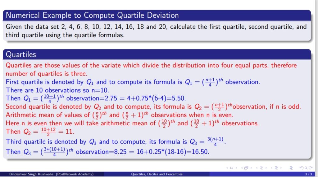
quartilenumerical2
Video
Conclusion
That’s it for today! Now you know how to calculate quartiles step-by-step. If you want to dive deeper into data analysis or have any questions, feel free to leave a comment below. Thank you for learning with me, Bindeshwar, at **Postnetwork Academy**. Stay tuned for more tutorials and helpful math tips!
This post explains how to calculate quartiles in a simple and understandable way. Use these methods to improve your data analysis skills and take your understanding of statistics to the next level!
