Chi Square Distribution

Chi Square Distribution

Chi square variate is a square of a normal variate having 1 degree of freedom and  chi square distribution is a special case of Gamma distribution.

If X is following normal distribution N(μ, σ) then Z=((X-μ)/σ)2 is a chi-square variate with 1 degree of freedom.

The generalized form of chi-square variate is that if X_i are normal variate independently distribute with means μ_i and variances σ_i.

Then the general form of chi squared can be written as with k degrees of freedom as.

Chi-squared distribution is very popular for statistical hypothesis testing such as goodness of fit. Chi-squared distribution has lot of applications in machine learning and data science for example, Chi-Squared Automatic Interaction Detection (CHAID) is a very popular chi-squared based decision tree learning algorithm.

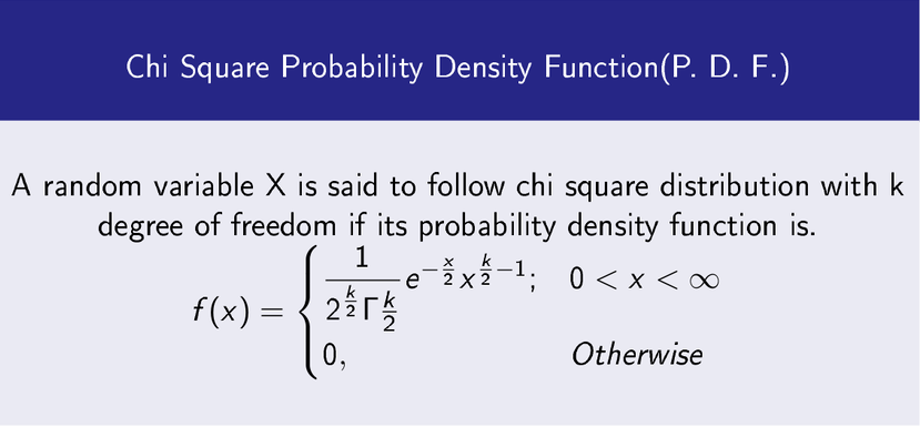
Chi-Squared Probability Density Function

The Probability Density Function (P. D. F.) of chi-squared distribution is given by.

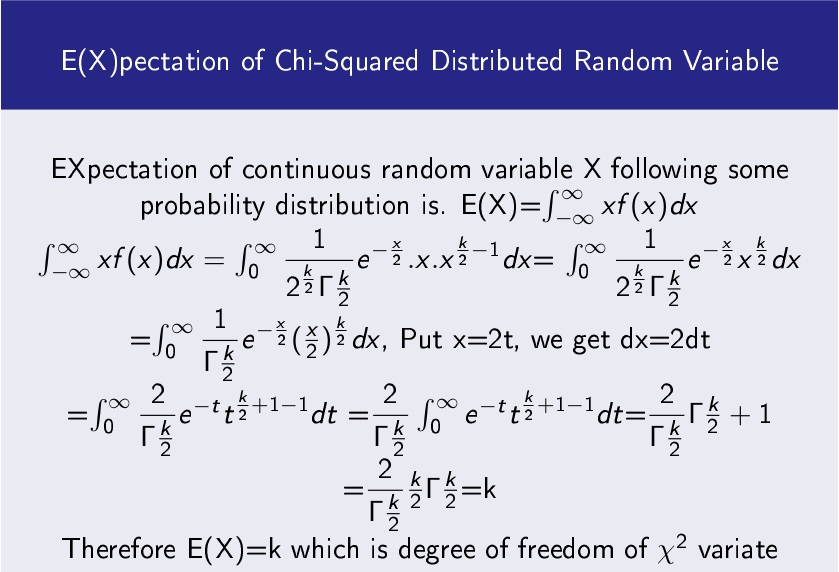
Expectation of Chi-Squared Distributed Random Variable

Expectation of chi-squared distributed random variable is calculated as follows.

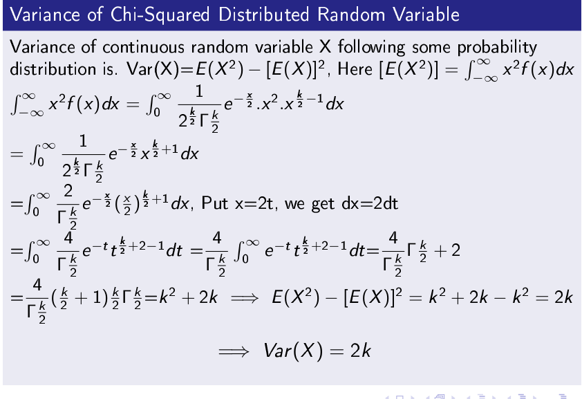
Variance of Chi-Squared Distributed Random Variable

Variance of chi-squared distributed random variable is calculated as follows.

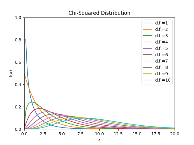
Plotting Chi-Squared Distribution with Different Degrees of Freedoms

---

import matplotlib.pyplot as plt
from scipy import stats
import numpy as np

1. x = np.linspace(0, 20, 100)

plt.plot(x, stats.chi2.pdf(x, 1), linestyle=’-‘,label=’d.f.=1’)
plt.plot(x, stats.chi2.pdf(x, 2), linestyle=’-‘, label=’d.f.=2’)
plt.plot(x, stats.chi2.pdf(x, 3), linestyle=’-‘, label=’d.f.=3’)
plt.plot(x, stats.chi2.pdf(x, 4), linestyle=’-‘, label=’d.f.=4’)
plt.plot(x, stats.chi2.pdf(x, 5), linestyle=’-‘, label=’d.f.=5’)
plt.plot(x, stats.chi2.pdf(x, 6), linestyle=’-‘, label=’d.f.=6’)
plt.plot(x, stats.chi2.pdf(x, 7), linestyle=’-‘, label=’d.f.=7’)
plt.plot(x, stats.chi2.pdf(x, 8), linestyle=’-‘, label=’d.f.=8’)
plt.plot(x, stats.chi2.pdf(x, 9), linestyle=’-‘, label=’d.f.=9’)
plt.plot(x, stats.chi2.pdf(x, 10), linestyle=’-‘, label=’d.f.=10’)

plt.xlim(0, 20)
plt.ylim(0, 1.0)

plt.xlabel(‘x’)
plt.ylabel(‘f(x)’)
plt.title(‘Chi-Squared Distribution’)
plt.legend()
plt.savefig(“Chi-Squared.png”)

---

 

From the above plot you can observe that if degree of freedom is low curve is highly right skewed. However, if degree of freedom increases it skewness is reduced and curve tends to be normal  curve, this also shows central limit theorem.

 

References

• Lancaster, H.O. and Seneta, E., 2005. Chi‐square distribution. Encyclopedia of biostatistics, 2.
• Canal, L., 2005. A normal approximation for the chi-square distribution. Computational statistics & data analysis, 48(4), pp.803-808.
• Kass, G.V., 1980. An exploratory technique for investigating large quantities of categorical data. Journal of the Royal Statistical Society: Series C (Applied Statistics), 29(2), pp.119-127.